\[\newcommand{\N}{\mathbb N}
\newcommand{\Z}{\mathbb Z}
\newcommand{\Q}{\mathbb Q}
\newcommand{\R}{\mathbb R}
\newcommand{\C}{\mathbb C}
\newcommand{\ba}{\mathbf{a}}
\newcommand{\bb}{\mathbf{b}}
\newcommand{\bc}{\mathbf{c}}
\newcommand{\bd}{\mathbf{d}}
\newcommand{\be}{\mathbf{e}}
\newcommand{\bff}{\mathbf{f}}
\newcommand{\bh}{\mathbf{h}}
\newcommand{\bi}{\mathbf{i}}
\newcommand{\bj}{\mathbf{j}}
\newcommand{\bk}{\mathbf{k}}
\newcommand{\bN}{\mathbf{N}}
\newcommand{\bn}{\mathbf{n}}
\newcommand{\bo}{\mathbf{0}}
\newcommand{\bp}{\mathbf{p}}
\newcommand{\bq}{\mathbf{q}}
\newcommand{\br}{\mathbf{r}}
\newcommand{\bs}{\mathbf{s}}
\newcommand{\bT}{\mathbf{T}}
\newcommand{\bu}{\mathbf{u}}
\newcommand{\bv}{\mathbf{v}}
\newcommand{\bw}{\mathbf{w}}
\newcommand{\bx}{\mathbf{x}}
\newcommand{\by}{\mathbf{y}}
\newcommand{\bz}{\mathbf{z}}
\newcommand{\bzero}{\mathbf{0}}
\newcommand{\nv}{\mathbf{0}}
\newcommand{\cA}{\mathcal{A}}
\newcommand{\cB}{\mathcal{B}}
\newcommand{\cC}{\mathcal{C}}
\newcommand{\cD}{\mathcal{D}}
\newcommand{\cE}{\mathcal{E}}
\newcommand{\cF}{\mathcal{F}}
\newcommand{\cG}{\mathcal{G}}
\newcommand{\cH}{\mathcal{H}}
\newcommand{\cI}{\mathcal{I}}
\newcommand{\cJ}{\mathcal{J}}
\newcommand{\cK}{\mathcal{K}}
\newcommand{\cL}{\mathcal{L}}
\newcommand{\cM}{\mathcal{M}}
\newcommand{\cN}{\mathcal{N}}
\newcommand{\cO}{\mathcal{O}}
\newcommand{\cP}{\mathcal{P}}
\newcommand{\cQ}{\mathcal{Q}}
\newcommand{\cR}{\mathcal{R}}
\newcommand{\cS}{\mathcal{S}}
\newcommand{\cT}{\mathcal{T}}
\newcommand{\cU}{\mathcal{U}}
\newcommand{\cV}{\mathcal{V}}
\newcommand{\cW}{\mathcal{W}}
\newcommand{\cX}{\mathcal{X}}
\newcommand{\cY}{\mathcal{Y}}
\newcommand{\cZ}{\mathcal{Z}}
\newcommand{\rA}{\mathrm{A}}
\newcommand{\rB}{\mathrm{B}}
\newcommand{\rC}{\mathrm{C}}
\newcommand{\rD}{\mathrm{D}}
\newcommand{\rE}{\mathrm{E}}
\newcommand{\rF}{\mathrm{F}}
\newcommand{\rG}{\mathrm{G}}
\newcommand{\rH}{\mathrm{H}}
\newcommand{\rI}{\mathrm{I}}
\newcommand{\rJ}{\mathrm{J}}
\newcommand{\rK}{\mathrm{K}}
\newcommand{\rL}{\mathrm{L}}
\newcommand{\rM}{\mathrm{M}}
\newcommand{\rN}{\mathrm{N}}
\newcommand{\rO}{\mathrm{O}}
\newcommand{\rP}{\mathrm{P}}
\newcommand{\rQ}{\mathrm{Q}}
\newcommand{\rR}{\mathrm{R}}
\newcommand{\rS}{\mathrm{S}}
\newcommand{\rT}{\mathrm{T}}
\newcommand{\rU}{\mathrm{U}}
\newcommand{\rV}{\mathrm{V}}
\newcommand{\rW}{\mathrm{W}}
\newcommand{\rX}{\mathrm{X}}
\newcommand{\rY}{\mathrm{Y}}
\newcommand{\rZ}{\mathrm{Z}}
\newcommand{\pv}{\overline}
\newcommand{\iu}{\mathrm{i}}
\newcommand{\ju}{\mathrm{j}}
\newcommand{\im}{\mathrm{i}}
\newcommand{\e}{\mathrm{e}}
\newcommand{\real}{\operatorname{Re}}
\newcommand{\imag}{\operatorname{Im}}
\newcommand{\Arg}{\operatorname{Arg}}
\newcommand{\Ln}{\operatorname{Ln}}
\DeclareMathOperator*{\res}{res}
\newcommand{\re}{\operatorname{Re}}
\newcommand{\im}{\operatorname{Im}}
\newcommand{\arsinh}{\operatorname{ar\,sinh}}
\newcommand{\arcosh}{\operatorname{ar\,cosh}}
\newcommand{\artanh}{\operatorname{ar\,tanh}}
\newcommand{\sgn}{\operatorname{sgn}}
\newcommand{\diag}{\operatorname{diag}}
\newcommand{\proj}{\operatorname{proj}}
\newcommand{\rref}{\operatorname{rref}}
\newcommand{\rank}{\operatorname{rank}}
\newcommand{\Span}{\operatorname{span}}
\newcommand{\vir}{\operatorname{span}}
\renewcommand{\dim}{\operatorname{dim}}
\newcommand{\alg}{\operatorname{alg}}
\newcommand{\geom}{\operatorname{geom}}
\newcommand{\id}{\operatorname{id}}
\newcommand{\norm}[1]{\lVert #1 \rVert}
\newcommand{\tp}[1]{#1^{\top}}
\renewcommand{\d}{\mathrm{d}}
\newcommand{\sij}[2]{\bigg/_{\mspace{-15mu}#1}^{\,#2}}
\newcommand{\abs}[1]{\lvert#1\rvert}
\newcommand{\pysty}[1]{\left[\begin{array}{@{}r@{}}#1\end{array}\right]}
\newcommand{\piste}{\cdot}
\newcommand{\qedhere}{}
\newcommand{\taumatrix}[1]{\left[\!\!#1\!\!\right]}
\newenvironment{augmatrix}[1]{\left[\begin{array}{#1}}{\end{array}\right]}
\newenvironment{vaugmatrix}[1]{\left|\begin{array}{#1}}{\end{array}\right|}
\newcommand{\trans}{\mathrm{T}}
\newcommand{\EUR}{\text{\unicode{0x20AC}}}
\newcommand{\SI}[3][]{#2\,\mathrm{#3}}
\newcommand{\si}[2][]{\mathrm{#2}}
\newcommand{\num}[2][]{#2}
\newcommand{\ang}[2][]{#2^{\circ}}
\newcommand{\meter}{m}
\newcommand{\metre}{\meter}
\newcommand{\kilo}{k}
\newcommand{\kilogram}{kg}
\newcommand{\gram}{g}
\newcommand{\squared}{^2}
\newcommand{\cubed}{^3}
\newcommand{\minute}{min}
\newcommand{\hour}{h}
\newcommand{\second}{s}
\newcommand{\degreeCelsius}{^{\circ}C}
\newcommand{\per}{/}
\newcommand{\centi}{c}
\newcommand{\milli}{m}
\newcommand{\deci}{d}
\newcommand{\percent}{\%}
\newcommand{\Var}{\operatorname{Var}}
\newcommand{\Cov}{\operatorname{Cov}}
\newcommand{\Corr}{\operatorname{Corr}}
\newcommand{\Tasd}{\operatorname{Tasd}}
\newcommand{\Ber}{\operatorname{Ber}}
\newcommand{\Bin}{\operatorname{Bin}}
\newcommand{\Geom}{\operatorname{Geom}}
\newcommand{\Poi}{\operatorname{Poi}}
\newcommand{\Hyperg}{\operatorname{Hyperg}}
\newcommand{\Tas}{\operatorname{Tas}}
\newcommand{\Exp}{\operatorname{Exp}}
\newcommand{\tdist}{\operatorname{t}}
\newcommand{\rd}{\mathrm{d}}
\newcommand{\oiint}{\unicode{x222F}}\]
Käyrä napakoordinaateissa
Tutkitaan vielä lyhyesti kaaren pituuden laskemista
napakoordinaattien (polar coordinates) avulla.
Tason piste \((x,y)\) voidaan esittää napakoordinaattien \(r,\theta\) avulla
muodossa
\[x=r\cos \theta,\ y=r\sin \theta,\]
missä \(r\ge 0\) ja \(\theta\in \R\)
(tai \(\theta\in [0,2\pi]\) tai \(\theta\in [-\pi,\pi]\) ). Monia tasojoukkoja on helpompi käsitellä
napakoordinaattien kuin tavallisten \(xy\)-koordinaattien avulla. Esimerkiksi
\(R\)-säteisen ympyrän yhtälö napakoordinaateissa on muotoa \(r=R\).
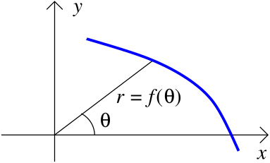
Tutkimme seuraavassa tasokäyrän \(r=f(\theta)\), \(\theta_0\le \theta \le \theta_1\),
kaaren pituuden laskemista. Tällainen käyrä voidaan parametrisoida kulman \(\theta = t\)
avulla, jolloin
\[\begin{split} \begin{cases}
x=r\cos \theta =f(\theta)\cos \theta =f(t)\cos t & \\
y=r\sin \theta =f(\theta)\sin \theta =f(t)\sin t. & \\
\end{cases}\end{split}\]
Tällöin
\[\br'(t)=(f'(t)\cos t-f(t)\sin t)\bi+(f'(t)\sin t+f(t)\cos t)\bj\]
ja \(\|\br'(t)\|=\sqrt{f(t)^2+f'(t)^2}\) sievennnysten jälkeen. Kaarenpituus saadaan
siis integraalista
\[\ell = \int_{\theta_0}^{\theta_1} \sqrt{f(t)^2+f'(t)^2}\, dt.\]
Esimerkki 2.6.1
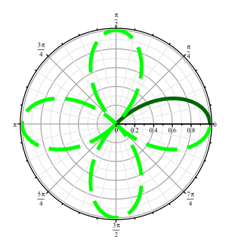
Laske neliapilan \(r=|\cos 2\theta|\), \(0\le \theta \le 2\pi\), kaarenpituus. (Useissa piirto-ohjelmissa lausekkeen voi kirjoittaa
myös ilman itseisarvoja ja kuva näyttää aivan samalta. Tällöin tapaus \(r<0\) vastaa
peilausta origon suhteen ja ”lehtien” kiertojärjestys muuttuu.)
Piilota/näytä ratkaisu
Symmetrian vuoksi riittää laskea kaarenpituus välillä \(\theta \in [0,\pi/4]\) ja
kertoa tulos luvulla 8. Tällöin myös \(\cos 2\theta \ge 0\), mikä helpottaa
laskuja.
Nyt siis \(f(t)=\cos 2t\) ja \(f'(t)=-2\sin 2t\), joten
kaarenpituudeksi saadaan
\[\ell = 8\int_0^{\pi/4} \sqrt{\cos^2(2t)+4\sin^2(2t)}\, dt =
8\int_0^{\pi/4} \sqrt{1+3\sin^2(2t)}\, dt \approx 9{,}69.\]
Kyseessä on ns. elliptinen
integraali, joka täytyy laskea numeerisesti; sillä ei ole alkeisfunktioiden
avulla esitettävää arvoa. Tämä ilmiö toistuu useissa kaarenpituuteen liittyvissä laskuissa.
Kappaleen loppuosa on oheislukemista.
Esimerkin 2.1.3 parametrisointi sopii huonosti
planeettojen ellipsiratojen kuvaamiseen, koska tapauksessa \(a\neq b\) parametrin \(t\) geometrinen
tulkinta ei ole enää napakoordinaatiston kulma \(\theta\) eikä myöskään aika: sille
käytetään tähtitieteessä nimeä luonnollinen anomalia.
(true anomaly) Kun origo asetetaan ellipsin toiseen
polttopisteeseen, niin radan parametrisointi saadaan napakoordinaattien avulla muotoon
\[r=\frac{a(1-e^2)}{1+e\cos\theta},\]
jossa \(a>0\) on ellipsin pidemmän puoliakselin pituus ja \(0\le e<1\) on ellipsin
eksentrisyys (eccentricity): \(e=\sqrt{1-b^2/a^2}\), jos \(a>b\). (Katso esimerkiksi
Kepler orbit.)
Kuvassa \(a=5\), \(b=4\), jolloin polttopiste(id)en etäisyys ellipsin keskipisteestä on
\[c=ae= \sqrt{a^2-b^2}=\sqrt{5^2-4^2}=3.\]
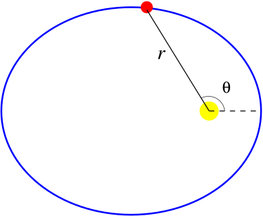
Aurinko ja punainen planeetta
Esimerkki 2.6.2
Tutki yhtälöiden
\(r=\frac{a(1-e^2)}{1+e\cos\theta}\ \text{ ja } \ \frac{(x-c)^2}{a^2}+\frac{y^2}{b^2}=1\)
välistä yhteyttä, kun \(e=\sqrt{1-b^2/a^2}<1\) ja \(c=ae\).
Piilota/näytä ratkaisu
Harjoitustehtävä.
Vihje: \(r=\sqrt{x^2+y^2}\) ja \(\cos(\arctan (y/x))=1/\sqrt{1+(y/x)^2}\).